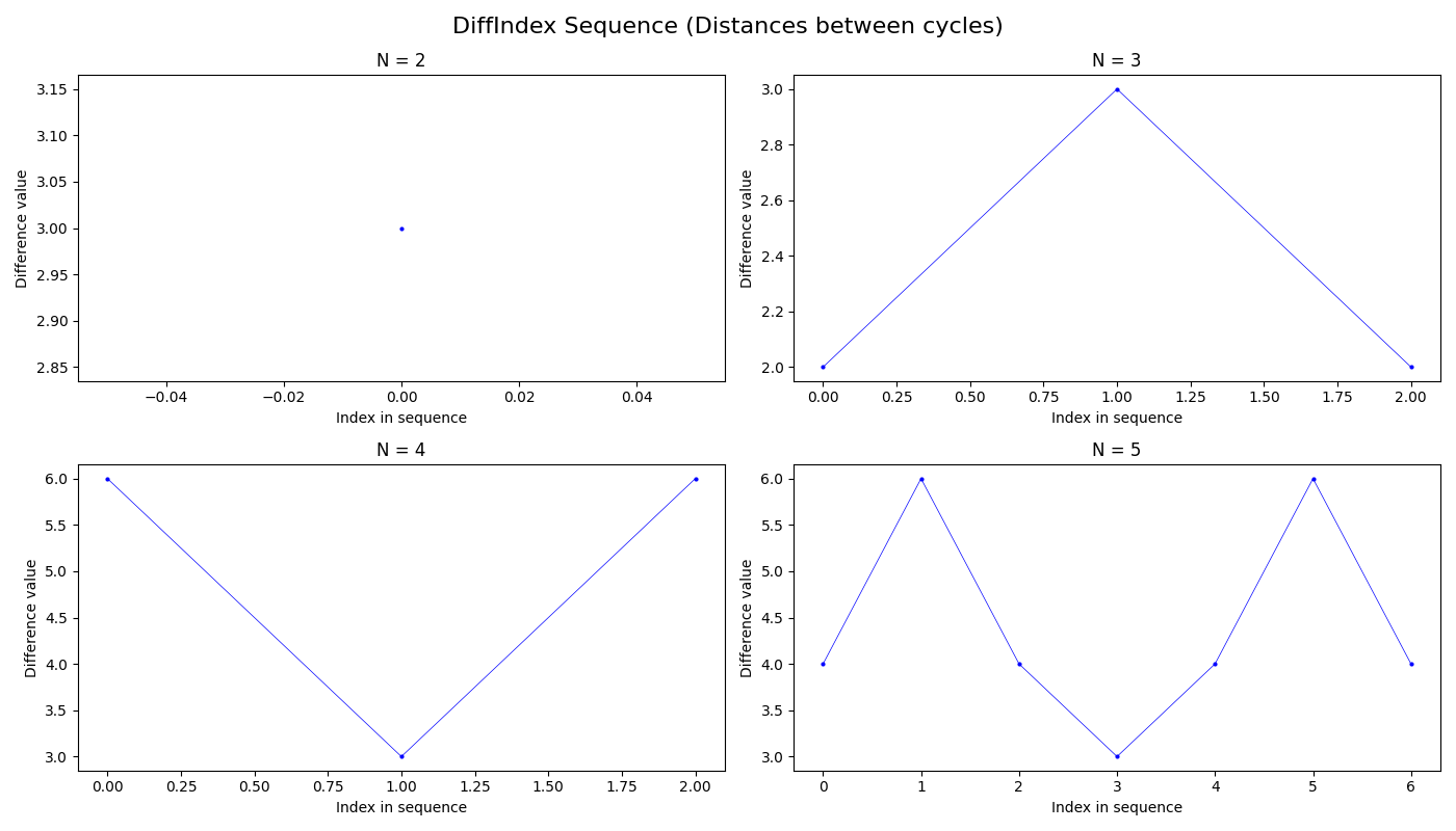
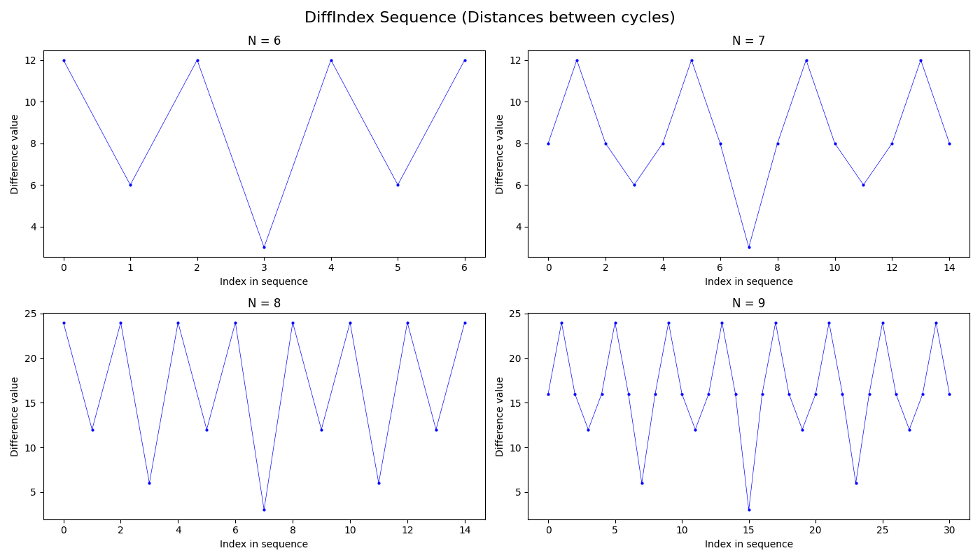
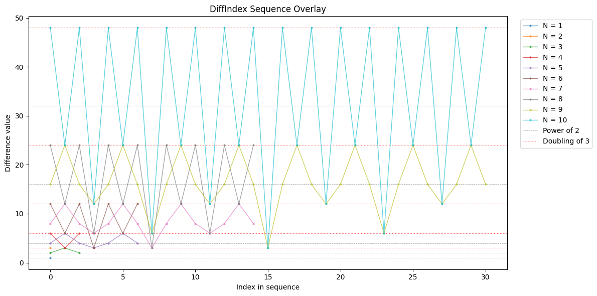
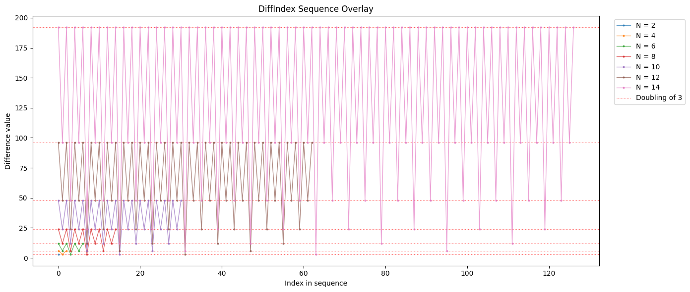
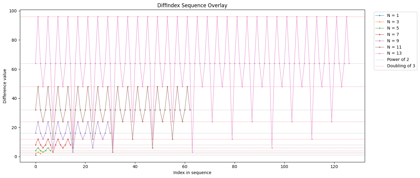
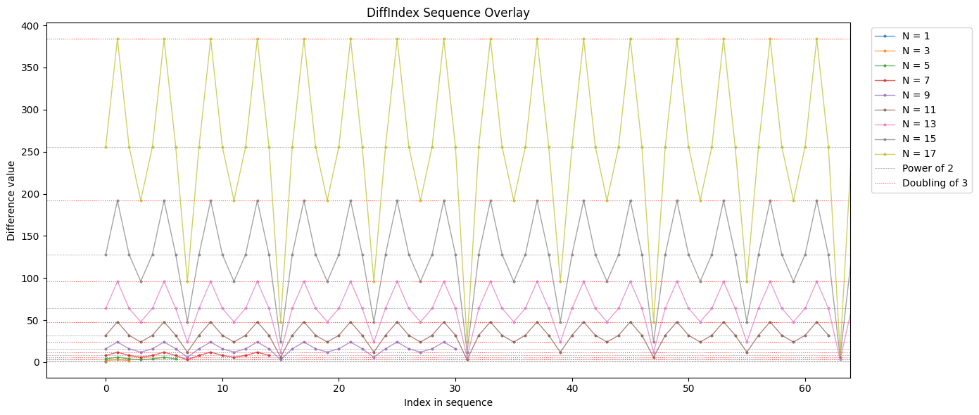
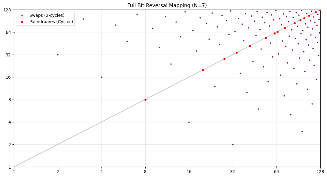
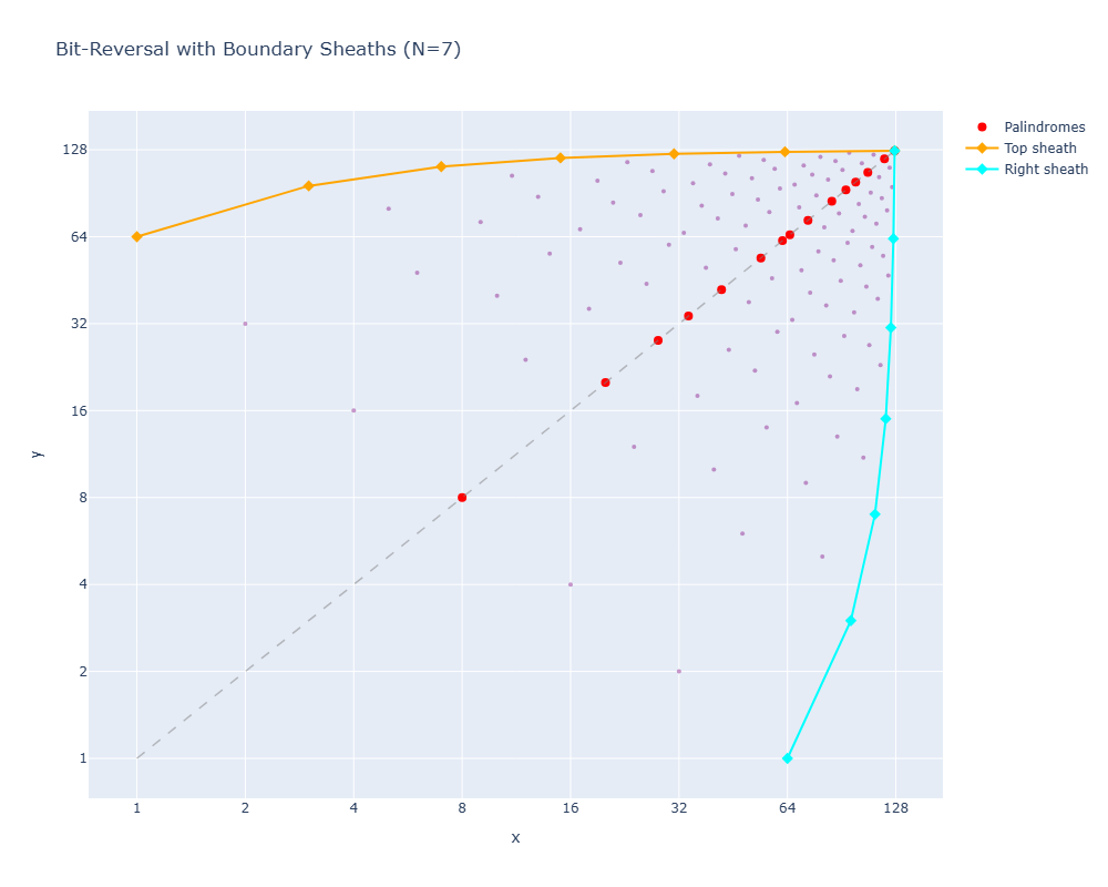
<?xml version="1.0" encoding="utf-8"?><feed xmlns="http://www.w3.org/2005/Atom" xml:lang="en"><generator uri="https://jekyllrb.com/" version="4.4.1">Jekyll</generator><link href="https://khilavm.github.io/feed.xml" rel="self" type="application/atom+xml"/><link href="https://khilavm.github.io/" rel="alternate" type="text/html" hreflang="en"/><updated>2026-07-27T20:29:14+00:00</updated><id>https://khilavm.github.io/feed.xml</id><title type="html">blank</title><subtitle>A simple, whitespace theme for academics. Based on [*folio](https://github.com/bogoli/-folio) design. </subtitle><entry><title type="html">More on bit-reversal</title><link href="https://khilavm.github.io/blog/2026/bit-reversal-cycles/" rel="alternate" type="text/html" title="More on bit-reversal"/><published>2026-05-01T06:00:00+00:00</published><updated>2026-05-01T06:00:00+00:00</updated><id>https://khilavm.github.io/blog/2026/bit-reversal-cycles</id><content type="html" xml:base="https://khilavm.github.io/blog/2026/bit-reversal-cycles/"><![CDATA[<h2 id="introduction">Introduction</h2> <p>Carrying on from the Danielson-Lanczos notes, we will discuss some interesting aspects of bit reversal here. We will consider all binary numbers that can be formed with \(N\) bits, calling it the set \(S(N)\). So,</p> \[\begin{align*} &amp; S(0)=\Phi \\ &amp; S(1)=\{0,1\} \\ &amp; S(2)=\{00,01,10,11\}_2=\{0,1,2,3\}_{10} \dots \end{align*}\] <p>where the subscript denotes the base of the set. This will be omitted further below where the distinction is obvious. Now denote by \(R_N\) the action of bit-reversal applied to \(S(N)\), i.e., \(R_N=\)<code class="language-plaintext highlighter-rouge">Rev</code>\((S(N))\). A key property of bit-reversal is that it is an <em>involution</em>: reversing twice returns the original number, so \(\texttt{Rev}(\texttt{Rev}(x))=x\) for all \(x \in S(N)\). This means every element either maps to itself (a fixed point) or belongs to a pair \(\{x,\texttt{Rev}(x)\}\) that swaps under reversal. Much of the structure that we discuss in this document follows from this fact.</p> \[\begin{align*} R_0&amp;=\Phi \\ R_1&amp;=\{0,1\} \\ R_2&amp;=\{00,10,01,11\}_2=\{0,2,1,3\}_{10} \\ R_3&amp;=\text{Rev}(\{000,001,010,011,100,101,110,111\}_2) \\ &amp;=\{000,100,010,110,001,101,011,111\}_2=\{0,4,2,6,1,5,3,7\}_{10} \\ R_4&amp;=\{0,8,4,12,2,10,6,14,1,9,5,13,3,11,7,15\}_{10} \dots \end{align*}\] <p>There are some things to notice here. First, that some numbers reverse to themselves. \(R_2(3)\), \(R_3(2)\) and \(R_4(17)\) are some of them. By \(R_N(p)\) we mean the \(p\)-th element of the set with indexing starting from \(0\). Second, that every \(R_N\) can be formed from \(R_{N-1}\) by a simple procedure that has been explained in the earlier document on the Danielson-Lanczos method. To construct the bit-reversed array for \(N=p\), take the one for \(N=p/2\) and after each element \(i\), insert an index \(2^{N-1}\). We will rewrite the arrays given above but with the new elements colored red. The elements in black are carried over from the previous \(N\).</p> \[\begin{align} &amp; N=1 \implies \{0,1\} \nonumber \\ &amp; N=2 \implies \{0,{\color{red}{2}},1,{\color{red}{3}}\} \nonumber \\ &amp; N=3 \implies \{0,{\color{red}{4}},2,{\color{red}{6}},1,{\color{red}{5}},3,{\color{red}{7}}\} \nonumber \\ &amp; N=4 \implies \{0,{\color{red}{8}},4,{\color{red}{12}},2,{\color{red}{10}},6,{\color{red}{14}},1,{\color{red}{9}},5,{\color{red}{13}},3,{\color{red}{11}},7,{\color{red}{15}}\} \label{cycred} \end{align}\] <h2 id="cycles">Cycles</h2> <p>Coming back to the first point, let us call the points that reverse to themselves <em>cycles</em>.<sup id="fnref:1"><a href="#fn:1" class="footnote" rel="footnote" role="doc-noteref">1</a></sup> Also, denote the set of cycles of \(R_N\) by \(C_N\). Thus,</p> \[\begin{align*} C_0&amp;=\Phi \\ C_1&amp;=\{0,1\} \\ C_2&amp;=\{0,3\} \\ C_3&amp;=\{0,2,5,7\} \\ C_4&amp;=\{0,6,9,15\} \\ C_5&amp;=\{0,4,10,14,17,21,27,31\} \\ C_6&amp;=\{0,12,18,30,33,45,51,63\} \\ C_7&amp;=\{0,8,20,28,34,42,54,62,65,73,85,93,99,107,109,127\} \\ C_8&amp;=\{0,24,36,60,66,90,102,126,129,153,165,189,195,219,231,255\} \end{align*}\] <p>Cycles can be found by simply finding the symmetric binary numbers for a certain \(N\). We are interested in where these cycles occur in \(R_N\). To see this, we will color the cycles in blue in the sets below.</p> \[\begin{align} R_1&amp;= \{ {\color{blue}{0}},1\} \nonumber \\ R_2&amp;= \{ {\color{blue}{0}},2,1,{\color{blue}{3}}\} \nonumber \\ R_3&amp;= \{ {\color{blue}{0}},4,{\color{blue}{2}},6,1,{\color{blue}{5}},3,{\color{blue}{7}}\} \nonumber \\ R_4&amp;= \{ {\color{blue}{0}},8,4,12,2,10,{\color{blue}{6}},14,1,{\color{blue}{9}},5,13,3,11,7,{\color{blue}{15}}\} \nonumber \\ R_5&amp;= \{ {\color{blue}{0}},16,8,24,{\color{blue}{4}},20,12,28,2,18,{\color{blue}{10}},26,6,22,{\color{blue}{14}},30,1,{\color{blue}{17}},9,25,5,{\color{blue}{21}},13,29,3,19,11,{\color{blue}{27}},7,23,15,{\color{blue}{31}}\} \label{r_blue} \end{align}\] <p>Obviously, \(R_N(2^{N-1})=1\) and \(R_N(1)=2^{N-1}\). The two trivial cycles are \(0\dots0\) and \(1\dots1\), which are the first and last elements. One can also spot easily the cycles \(100\dots001\) and \(011\dots110\). The former is two places before the “central” \(1\) and the latter right after it. See the elements \(R_N(2^{N-1}-2)\) and \(R_N(2^{N-1}+1)\) in the above sets. For example, \({\color{blue}{14}}\) and \({\color{blue}{17}}\) in \(R_5\), and \({\color{blue}{6}}\) and \({\color{blue}{9}}\) in \(R_4\).</p> <p>How many cycles are present in \(R_N\)? By counting up to \(N=8\), we get the following table.</p> <table> <thead> <tr> <th style="text-align: center"><strong>N</strong></th> <th style="text-align: center"><strong>Cycles</strong></th> <th style="text-align: center"><strong>N</strong></th> <th style="text-align: center"><strong>Cycles</strong></th> </tr> </thead> <tbody> <tr> <td style="text-align: center">1</td> <td style="text-align: center">2</td> <td style="text-align: center">5</td> <td style="text-align: center">8</td> </tr> <tr> <td style="text-align: center">2</td> <td style="text-align: center">2</td> <td style="text-align: center">6</td> <td style="text-align: center">8</td> </tr> <tr> <td style="text-align: center">3</td> <td style="text-align: center">4</td> <td style="text-align: center">7</td> <td style="text-align: center">16</td> </tr> <tr> <td style="text-align: center">4</td> <td style="text-align: center">4</td> <td style="text-align: center">8</td> <td style="text-align: center">16</td> </tr> </tbody> </table> <p>Let us denote the number of cycles in \(R_N\), or the number of elements in \(C_N\), as \(\mathcal{N}_N\). We may conjecture that if \(N\) is even, then \(\mathcal{N}_N=2^{N/2}\), and if \(N\) is odd, then \(\mathcal{N}_N=2^{(N+1)/2}\). This can easily be verified by looking at binary numbers in \(5\) and \(6\) bits. Take \(00100\). Finding a cycle under bit-reversal is equivalent to fixing the middle element — the 1 here — and folding one side onto the other. The elements to the left of the middle one can be chosen in \(2^{(N-1)/2}\) ways, and the middle element can be either \(0\) or \(1\). So, multiplying by two gives \(\mathcal{N}_{N\text{ odd}}=2^{(N+1)/2}\). For the even \(N\) case, consider \(001100\). Here it is merely a question of folding straight down the middle, so we only need to choose our bits on one side, giving \(\mathcal{N}_{N\text{ even}}=2^{N/2}\). Combining both odd and even cases, we can write the number of cycles for \(N\) bits as \(\mathcal{N}_N=2^{\lceil N/2 \rceil}\). This sequence \(\{2,2,4,4,8,8,16,16,\dots\}\) appears in the On-Line Encyclopedia of Integer Sequences (OEIS) as <a href="https://oeis.org/A060546">A060546</a>. A consequence of the involution property is that the remaining \(2^N - \mathcal{N}_N\) elements pair off into 2-cycles, so the total number of 2-cycles is \((2^N - 2^{\lceil N/2 \rceil})/2\).</p> <h2 id="distribution">Distribution</h2> <p>How are the cycles distributed in \(R_N\)? We have already noted the locations of the trivial ones at the two ends of the set and the two close to the “central” \(1\). Let us write down the number of elements <strong>between</strong> consecutive cycles for the first few \(N\)’s, represented by <strong>Distances</strong> in the table below.</p> <table> <thead> <tr> <th style="text-align: center"><strong>N</strong></th> <th style="text-align: left"><strong>Distances</strong></th> <th style="text-align: center"><strong>N</strong></th> <th style="text-align: left"><strong>Distances</strong></th> </tr> </thead> <tbody> <tr> <td style="text-align: center">1</td> <td style="text-align: left">0</td> <td style="text-align: center">5</td> <td style="text-align: left">3,5,3,2,3,5,3</td> </tr> <tr> <td style="text-align: center">2</td> <td style="text-align: left">2</td> <td style="text-align: center">6</td> <td style="text-align: left">11,5,11,2,11,5,11</td> </tr> <tr> <td style="text-align: center">3</td> <td style="text-align: left">1,2,1</td> <td style="text-align: center">7</td> <td style="text-align: left">7,11,7,5,7,11,7,2,7,11,7,5,7,11,7</td> </tr> <tr> <td style="text-align: center">4</td> <td style="text-align: left">5,2,5</td> <td style="text-align: center">8</td> <td style="text-align: left">23,11,23,5,23,11,23,2,23,11,23,5,23,11,23</td> </tr> </tbody> </table> <p>We see that the distances between consecutive cycles are symmetric about the middle distance of 2. It may be more useful to write the distances as a mere difference of their position indices, which would increase values in the table above by \(1\). We represent this distance by <strong>DiffIndex</strong>. The symmetric part to the right of the central distance is denoted by an ellipsis.</p> <table> <thead> <tr> <th style="text-align: center"><strong>N</strong></th> <th style="text-align: left"><strong>DiffIndex</strong></th> <th style="text-align: center"><strong>N</strong></th> <th style="text-align: left"><strong>DiffIndex</strong></th> </tr> </thead> <tbody> <tr> <td style="text-align: center">1</td> <td style="text-align: left">0</td> <td style="text-align: center">5</td> <td style="text-align: left">4,6,4,3,…</td> </tr> <tr> <td style="text-align: center">2</td> <td style="text-align: left">3</td> <td style="text-align: center">6</td> <td style="text-align: left">12,6,12,3,…</td> </tr> <tr> <td style="text-align: center">3</td> <td style="text-align: left">2,3,…</td> <td style="text-align: center">7</td> <td style="text-align: left">8,12,8,6,8,12,8,3,…</td> </tr> <tr> <td style="text-align: center">4</td> <td style="text-align: left">6,3,…</td> <td style="text-align: center">8</td> <td style="text-align: left">24,12,24,6,24,12,24,3,…</td> </tr> </tbody> </table> <p>We are beginning to see some kind of structure. Apart from the central distance of \(3\), we see a doubling for each \((2k-1,2k)\) pair. Now look at the progression from \(N=3\) to \(N=5\) to \(N=7\). We see that we can take a mirror image around the central \(3\), multiply all distances by \(2\), reappend the central \(3\) at the end of that sequence to obtain the next set of differences. Thus, to get the \(N=7\) set, take the \(N=5\) one of \(4,6,4,3,\dots\). Mirroring about \(3\) gives \(4,6,4,3,4,6,4\). Doubling leads to \(8,12,8,6,8,12,8\). This gives the first set of distances. To generate the full set, we just need to mirror it after crossing the central distance of \(3\), giving \(8,12,8,6,8,12,8,3,\dots\). The same logic holds for going from \(N=4\) to \(N=6\) to \(N=8\).</p> <p>Now look at the value of the first nontrivial cycle for a \((2k-1,2k)\) pair. You will see that there is a tripling. Why? What is the smallest cycle we can form after \(0\dots0\)? Writing down all possible cycles as we will show below for a couple of cases, we will see that it is the binary number with all zeroes except a one in the middle when \(N\) is odd and two ones in the middle when \(N\) is even. Their values in base \(10\) are \(2^{(N-1)/2}\) for the former and \(2^{N/2}\) for the latter. Taking the difference of these two numbers gives us \(3(2^{(N-1)/2})\), which is triple the one for \(N=2k-1\).</p> <h2 id="generating-cycles">Generating cycles</h2> <p>Let us now write down the cycles for \(N=7\) and \(N=8\) in both binary and base \(10\). Look at the \(N=7\) table first. Note that the central bit in the binary numbers alternates between \(0\) and \(1\). For every consecutive \(0,1\) pair, we have the same 3-bit binary number — underlined in green in the tables below — which is mirrored about the central element to make the cycle. What is the value of this underlined binary in base \(10\)? It is shown in blue in the tables below. Now look at equation \eqref{r_blue}! These are exactly the values in our bit-reversed arrays \(R_N\)! For odd \(N\), we reproduce the array \(R_{(N-1)/2}\) and for even \(N\) we get \(R_{N/2}\). There is no central bit for \(N=8\) so the mirror is simply in the middle of the binary sequence.</p> <div class="row mt-3"> <div class="col-md-6"> <p style="text-align:center"><strong>(a) N=7</strong></p> <table class="cycle-table"> <thead><tr><th>C(10)</th><th>C(2)</th><th>C(10)</th><th>C(2)</th></tr></thead> <tbody> <tr><td>0</td><td><span class="bv">000<span class="bv-brown">0</span><span class="bv-green-ul">000</span></span> (<span class="bv-blue">0</span>)</td><td>65</td><td><span class="bv">100<span class="bv-brown">0</span><span class="bv-green-ul">001</span></span> (<span class="bv-blue">1</span>)</td></tr> <tr><td>8</td><td><span class="bv">000<span class="bv-brown">1</span><span class="bv-green-ul">000</span></span> (<span class="bv-blue">0</span>)</td><td>73</td><td><span class="bv">100<span class="bv-brown">1</span><span class="bv-green-ul">001</span></span> (<span class="bv-blue">1</span>)</td></tr> <tr><td>20</td><td><span class="bv">001<span class="bv-brown">0</span><span class="bv-green-ul">100</span></span> (<span class="bv-blue">4</span>)</td><td>85</td><td><span class="bv">101<span class="bv-brown">0</span><span class="bv-green-ul">101</span></span> (<span class="bv-blue">5</span>)</td></tr> <tr><td>28</td><td><span class="bv">001<span class="bv-brown">1</span><span class="bv-green-ul">100</span></span> (<span class="bv-blue">4</span>)</td><td>93</td><td><span class="bv">101<span class="bv-brown">1</span><span class="bv-green-ul">101</span></span> (<span class="bv-blue">5</span>)</td></tr> <tr><td>34</td><td><span class="bv">010<span class="bv-brown">0</span><span class="bv-green-ul">010</span></span> (<span class="bv-blue">2</span>)</td><td>99</td><td><span class="bv">110<span class="bv-brown">0</span><span class="bv-green-ul">011</span></span> (<span class="bv-blue">3</span>)</td></tr> <tr><td>42</td><td><span class="bv">010<span class="bv-brown">1</span><span class="bv-green-ul">010</span></span> (<span class="bv-blue">2</span>)</td><td>107</td><td><span class="bv">110<span class="bv-brown">1</span><span class="bv-green-ul">011</span></span> (<span class="bv-blue">3</span>)</td></tr> <tr><td>54</td><td><span class="bv">011<span class="bv-brown">0</span><span class="bv-green-ul">110</span></span> (<span class="bv-blue">6</span>)</td><td>119</td><td><span class="bv">111<span class="bv-brown">0</span><span class="bv-green-ul">111</span></span> (<span class="bv-blue">7</span>)</td></tr> <tr><td>62</td><td><span class="bv">011<span class="bv-brown">1</span><span class="bv-green-ul">110</span></span> (<span class="bv-blue">6</span>)</td><td>127</td><td><span class="bv">111<span class="bv-brown">1</span><span class="bv-green-ul">111</span></span> (<span class="bv-blue">7</span>)</td></tr> </tbody> </table> </div> <div class="col-md-6"> <p style="text-align:center"><strong>(b) N=8</strong></p> <table class="cycle-table"> <thead><tr><th>C(10)</th><th>C(2)</th><th>C(10)</th><th>C(2)</th></tr></thead> <tbody> <tr><td>0</td><td><span class="bv">0000<span class="bv-green-ul">0000</span></span> (<span class="bv-blue">0</span>)</td><td>129</td><td><span class="bv">1000<span class="bv-green-ul">0001</span></span> (<span class="bv-blue">1</span>)</td></tr> <tr><td>24</td><td><span class="bv">0001<span class="bv-green-ul">1000</span></span> (<span class="bv-blue">8</span>)</td><td>153</td><td><span class="bv">1001<span class="bv-green-ul">1001</span></span> (<span class="bv-blue">9</span>)</td></tr> <tr><td>36</td><td><span class="bv">0010<span class="bv-green-ul">0100</span></span> (<span class="bv-blue">4</span>)</td><td>165</td><td><span class="bv">1010<span class="bv-green-ul">0101</span></span> (<span class="bv-blue">5</span>)</td></tr> <tr><td>60</td><td><span class="bv">0011<span class="bv-green-ul">1100</span></span> (<span class="bv-blue">12</span>)</td><td>189</td><td><span class="bv">1011<span class="bv-green-ul">1101</span></span> (<span class="bv-blue">13</span>)</td></tr> <tr><td>66</td><td><span class="bv">0100<span class="bv-green-ul">0010</span></span> (<span class="bv-blue">2</span>)</td><td>195</td><td><span class="bv">1100<span class="bv-green-ul">0011</span></span> (<span class="bv-blue">3</span>)</td></tr> <tr><td>90</td><td><span class="bv">0101<span class="bv-green-ul">1010</span></span> (<span class="bv-blue">10</span>)</td><td>219</td><td><span class="bv">1101<span class="bv-green-ul">1011</span></span> (<span class="bv-blue">11</span>)</td></tr> <tr><td>102</td><td><span class="bv">0110<span class="bv-green-ul">0110</span></span> (<span class="bv-blue">6</span>)</td><td>231</td><td><span class="bv">1110<span class="bv-green-ul">0111</span></span> (<span class="bv-blue">7</span>)</td></tr> <tr><td>126</td><td><span class="bv">0111<span class="bv-green-ul">1110</span></span> (<span class="bv-blue">14</span>)</td><td>255</td><td><span class="bv">1111<span class="bv-green-ul">1111</span></span> (<span class="bv-blue">15</span>)</td></tr> </tbody> </table> </div> </div> <p class="text-center mt-2"><em>The central bit in (a) is colored brown, the bits to the right are underlined in green, and the decimal value of the underlined binary is shown in blue. There is no central bit in (b).</em></p> <p>The tables below show \(N=9\) and \(N=10\).</p> <div class="row mt-3"> <div class="col-md-6"> <p style="text-align:center"><strong>(a) N=9</strong></p> <table class="cycle-table"> <thead><tr><th>C(10)</th><th>C(2)</th><th>C(10)</th><th>C(2)</th></tr></thead> <tbody> <tr><td>0</td><td><span class="bv">0000<span class="bv-brown">0</span><span class="bv-green-ul">0000</span></span> (<span class="bv-blue">0</span>)</td><td>257</td><td><span class="bv">1000<span class="bv-brown">0</span><span class="bv-green-ul">0001</span></span> (<span class="bv-blue">1</span>)</td></tr> <tr><td>16</td><td><span class="bv">0000<span class="bv-brown">1</span><span class="bv-green-ul">0000</span></span> (<span class="bv-blue">0</span>)</td><td>273</td><td><span class="bv">1000<span class="bv-brown">1</span><span class="bv-green-ul">0001</span></span> (<span class="bv-blue">1</span>)</td></tr> <tr><td>40</td><td><span class="bv">0001<span class="bv-brown">0</span><span class="bv-green-ul">1000</span></span> (<span class="bv-blue">8</span>)</td><td>297</td><td><span class="bv">1001<span class="bv-brown">0</span><span class="bv-green-ul">1001</span></span> (<span class="bv-blue">9</span>)</td></tr> <tr><td>56</td><td><span class="bv">0001<span class="bv-brown">1</span><span class="bv-green-ul">1000</span></span> (<span class="bv-blue">8</span>)</td><td>313</td><td><span class="bv">1001<span class="bv-brown">1</span><span class="bv-green-ul">1001</span></span> (<span class="bv-blue">9</span>)</td></tr> <tr><td>68</td><td><span class="bv">0010<span class="bv-brown">0</span><span class="bv-green-ul">0100</span></span> (<span class="bv-blue">4</span>)</td><td>325</td><td><span class="bv">1010<span class="bv-brown">0</span><span class="bv-green-ul">0101</span></span> (<span class="bv-blue">5</span>)</td></tr> <tr><td>84</td><td><span class="bv">0010<span class="bv-brown">1</span><span class="bv-green-ul">0100</span></span> (<span class="bv-blue">4</span>)</td><td>341</td><td><span class="bv">1010<span class="bv-brown">1</span><span class="bv-green-ul">0101</span></span> (<span class="bv-blue">5</span>)</td></tr> <tr><td>108</td><td><span class="bv">0011<span class="bv-brown">0</span><span class="bv-green-ul">1100</span></span> (<span class="bv-blue">12</span>)</td><td>365</td><td><span class="bv">1011<span class="bv-brown">0</span><span class="bv-green-ul">1101</span></span> (<span class="bv-blue">13</span>)</td></tr> <tr><td>124</td><td><span class="bv">0011<span class="bv-brown">1</span><span class="bv-green-ul">1100</span></span> (<span class="bv-blue">12</span>)</td><td>381</td><td><span class="bv">1011<span class="bv-brown">1</span><span class="bv-green-ul">1101</span></span> (<span class="bv-blue">13</span>)</td></tr> <tr><td>130</td><td><span class="bv">0100<span class="bv-brown">0</span><span class="bv-green-ul">0010</span></span> (<span class="bv-blue">2</span>)</td><td>387</td><td><span class="bv">1100<span class="bv-brown">0</span><span class="bv-green-ul">0011</span></span> (<span class="bv-blue">3</span>)</td></tr> <tr><td>146</td><td><span class="bv">0100<span class="bv-brown">1</span><span class="bv-green-ul">0010</span></span> (<span class="bv-blue">2</span>)</td><td>403</td><td><span class="bv">1100<span class="bv-brown">1</span><span class="bv-green-ul">0011</span></span> (<span class="bv-blue">3</span>)</td></tr> <tr><td>170</td><td><span class="bv">0101<span class="bv-brown">0</span><span class="bv-green-ul">1010</span></span> (<span class="bv-blue">10</span>)</td><td>427</td><td><span class="bv">1101<span class="bv-brown">0</span><span class="bv-green-ul">1011</span></span> (<span class="bv-blue">11</span>)</td></tr> <tr><td>186</td><td><span class="bv">0101<span class="bv-brown">1</span><span class="bv-green-ul">1010</span></span> (<span class="bv-blue">10</span>)</td><td>443</td><td><span class="bv">1101<span class="bv-brown">1</span><span class="bv-green-ul">1011</span></span> (<span class="bv-blue">11</span>)</td></tr> <tr><td>198</td><td><span class="bv">0110<span class="bv-brown">0</span><span class="bv-green-ul">0110</span></span> (<span class="bv-blue">6</span>)</td><td>455</td><td><span class="bv">1110<span class="bv-brown">0</span><span class="bv-green-ul">0111</span></span> (<span class="bv-blue">7</span>)</td></tr> <tr><td>214</td><td><span class="bv">0110<span class="bv-brown">1</span><span class="bv-green-ul">0110</span></span> (<span class="bv-blue">6</span>)</td><td>471</td><td><span class="bv">1110<span class="bv-brown">1</span><span class="bv-green-ul">0111</span></span> (<span class="bv-blue">7</span>)</td></tr> <tr><td>238</td><td><span class="bv">0111<span class="bv-brown">0</span><span class="bv-green-ul">1110</span></span> (<span class="bv-blue">14</span>)</td><td>495</td><td><span class="bv">1111<span class="bv-brown">0</span><span class="bv-green-ul">1111</span></span> (<span class="bv-blue">15</span>)</td></tr> <tr><td>254</td><td><span class="bv">0111<span class="bv-brown">1</span><span class="bv-green-ul">1110</span></span> (<span class="bv-blue">14</span>)</td><td>511</td><td><span class="bv">1111<span class="bv-brown">1</span><span class="bv-green-ul">1111</span></span> (<span class="bv-blue">15</span>)</td></tr> </tbody> </table> </div> <div class="col-md-6"> <p style="text-align:center"><strong>(b) N=10</strong></p> <table class="cycle-table"> <thead><tr><th>C(10)</th><th>C(2)</th><th>C(10)</th><th>C(2)</th></tr></thead> <tbody> <tr><td>0</td><td><span class="bv">00000<span class="bv-green-ul">00000</span></span> (<span class="bv-blue">0</span>)</td><td>513</td><td><span class="bv">10000<span class="bv-green-ul">00001</span></span> (<span class="bv-blue">1</span>)</td></tr> <tr><td>48</td><td><span class="bv">00001<span class="bv-green-ul">10000</span></span> (<span class="bv-blue">16</span>)</td><td>561</td><td><span class="bv">10001<span class="bv-green-ul">10001</span></span> (<span class="bv-blue">17</span>)</td></tr> <tr><td>72</td><td><span class="bv">00010<span class="bv-green-ul">01000</span></span> (<span class="bv-blue">8</span>)</td><td>585</td><td><span class="bv">10010<span class="bv-green-ul">01001</span></span> (<span class="bv-blue">9</span>)</td></tr> <tr><td>120</td><td><span class="bv">00011<span class="bv-green-ul">11000</span></span> (<span class="bv-blue">24</span>)</td><td>633</td><td><span class="bv">10011<span class="bv-green-ul">11001</span></span> (<span class="bv-blue">25</span>)</td></tr> <tr><td>132</td><td><span class="bv">00100<span class="bv-green-ul">00100</span></span> (<span class="bv-blue">4</span>)</td><td>645</td><td><span class="bv">10100<span class="bv-green-ul">00101</span></span> (<span class="bv-blue">5</span>)</td></tr> <tr><td>180</td><td><span class="bv">00101<span class="bv-green-ul">10100</span></span> (<span class="bv-blue">20</span>)</td><td>693</td><td><span class="bv">10101<span class="bv-green-ul">10101</span></span> (<span class="bv-blue">21</span>)</td></tr> <tr><td>204</td><td><span class="bv">00110<span class="bv-green-ul">01100</span></span> (<span class="bv-blue">12</span>)</td><td>717</td><td><span class="bv">10110<span class="bv-green-ul">01101</span></span> (<span class="bv-blue">13</span>)</td></tr> <tr><td>252</td><td><span class="bv">00111<span class="bv-green-ul">11100</span></span> (<span class="bv-blue">28</span>)</td><td>765</td><td><span class="bv">10111<span class="bv-green-ul">11101</span></span> (<span class="bv-blue">29</span>)</td></tr> <tr><td>258</td><td><span class="bv">01000<span class="bv-green-ul">00010</span></span> (<span class="bv-blue">2</span>)</td><td>771</td><td><span class="bv">11000<span class="bv-green-ul">00011</span></span> (<span class="bv-blue">3</span>)</td></tr> <tr><td>306</td><td><span class="bv">01001<span class="bv-green-ul">10010</span></span> (<span class="bv-blue">18</span>)</td><td>819</td><td><span class="bv">11001<span class="bv-green-ul">10011</span></span> (<span class="bv-blue">19</span>)</td></tr> <tr><td>330</td><td><span class="bv">01010<span class="bv-green-ul">01010</span></span> (<span class="bv-blue">10</span>)</td><td>843</td><td><span class="bv">11010<span class="bv-green-ul">01011</span></span> (<span class="bv-blue">11</span>)</td></tr> <tr><td>378</td><td><span class="bv">01011<span class="bv-green-ul">11010</span></span> (<span class="bv-blue">26</span>)</td><td>891</td><td><span class="bv">11011<span class="bv-green-ul">11011</span></span> (<span class="bv-blue">27</span>)</td></tr> <tr><td>390</td><td><span class="bv">01100<span class="bv-green-ul">00110</span></span> (<span class="bv-blue">6</span>)</td><td>903</td><td><span class="bv">11100<span class="bv-green-ul">00111</span></span> (<span class="bv-blue">7</span>)</td></tr> <tr><td>438</td><td><span class="bv">01101<span class="bv-green-ul">10110</span></span> (<span class="bv-blue">22</span>)</td><td>951</td><td><span class="bv">11101<span class="bv-green-ul">10111</span></span> (<span class="bv-blue">23</span>)</td></tr> <tr><td>462</td><td><span class="bv">01110<span class="bv-green-ul">01110</span></span> (<span class="bv-blue">14</span>)</td><td>975</td><td><span class="bv">11110<span class="bv-green-ul">01111</span></span> (<span class="bv-blue">15</span>)</td></tr> <tr><td>510</td><td><span class="bv">01111<span class="bv-green-ul">11110</span></span> (<span class="bv-blue">30</span>)</td><td>1023</td><td><span class="bv">11111<span class="bv-green-ul">11111</span></span> (<span class="bv-blue">31</span>)</td></tr> </tbody> </table> </div> </div> <p class="text-center mt-2"><em>Cycles with decimal and binary values for N=9 and N=10.</em></p> <p>We see that to construct cycles for any even \(N\), we just need the bit-reversed array \(R_{N/2}\). A suitable mirroring of the elements of this set leads to \(C_N\). <strong>We don’t need to search for all symmetric combinations of bits</strong>. Similarly for odd \(N\). And thus we can write the generator of cycles for \(N\) bits as \(R_{\lfloor N/2 \rfloor}\). The tables below show similar cycles for \(N\in\{3,4,5,6\}\).</p> <div class="row mt-3"> <div class="col-md-6"> <p style="text-align:center"><strong>(a) N=3</strong></p> <table class="cycle-table"> <thead><tr><th>C(10)</th><th>C(2)</th></tr></thead> <tbody> <tr><td>0</td><td><span class="bv">0<span class="bv-brown">0</span><span class="bv-green-ul">0</span></span> (<span class="bv-blue">0</span>)</td></tr> <tr><td>2</td><td><span class="bv">0<span class="bv-brown">1</span><span class="bv-green-ul">0</span></span> (<span class="bv-blue">0</span>)</td></tr> <tr><td>5</td><td><span class="bv">1<span class="bv-brown">0</span><span class="bv-green-ul">1</span></span> (<span class="bv-blue">1</span>)</td></tr> <tr><td>7</td><td><span class="bv">1<span class="bv-brown">1</span><span class="bv-green-ul">1</span></span> (<span class="bv-blue">1</span>)</td></tr> </tbody> </table> </div> <div class="col-md-6"> <p style="text-align:center"><strong>(b) N=4</strong></p> <table class="cycle-table"> <thead><tr><th>C(10)</th><th>C(2)</th></tr></thead> <tbody> <tr><td>0</td><td><span class="bv">00<span class="bv-green-ul">00</span></span> (<span class="bv-blue">0</span>)</td></tr> <tr><td>6</td><td><span class="bv">01<span class="bv-green-ul">10</span></span> (<span class="bv-blue">2</span>)</td></tr> <tr><td>9</td><td><span class="bv">10<span class="bv-green-ul">01</span></span> (<span class="bv-blue">1</span>)</td></tr> <tr><td>15</td><td><span class="bv">11<span class="bv-green-ul">11</span></span> (<span class="bv-blue">3</span>)</td></tr> </tbody> </table> </div> </div> <div class="row mt-3"> <div class="col-md-6"> <p style="text-align:center"><strong>(a) N=5</strong></p> <table class="cycle-table"> <thead><tr><th>C(10)</th><th>C(2)</th></tr></thead> <tbody> <tr><td>0</td><td><span class="bv">00<span class="bv-brown">0</span><span class="bv-green-ul">00</span></span> (<span class="bv-blue">0</span>)</td></tr> <tr><td>4</td><td><span class="bv">00<span class="bv-brown">1</span><span class="bv-green-ul">00</span></span> (<span class="bv-blue">0</span>)</td></tr> <tr><td>10</td><td><span class="bv">01<span class="bv-brown">0</span><span class="bv-green-ul">10</span></span> (<span class="bv-blue">2</span>)</td></tr> <tr><td>14</td><td><span class="bv">01<span class="bv-brown">1</span><span class="bv-green-ul">10</span></span> (<span class="bv-blue">2</span>)</td></tr> <tr><td>17</td><td><span class="bv">10<span class="bv-brown">0</span><span class="bv-green-ul">01</span></span> (<span class="bv-blue">1</span>)</td></tr> <tr><td>21</td><td><span class="bv">10<span class="bv-brown">1</span><span class="bv-green-ul">01</span></span> (<span class="bv-blue">1</span>)</td></tr> <tr><td>27</td><td><span class="bv">11<span class="bv-brown">0</span><span class="bv-green-ul">11</span></span> (<span class="bv-blue">3</span>)</td></tr> <tr><td>31</td><td><span class="bv">11<span class="bv-brown">1</span><span class="bv-green-ul">11</span></span> (<span class="bv-blue">3</span>)</td></tr> </tbody> </table> </div> <div class="col-md-6"> <p style="text-align:center"><strong>(b) N=6</strong></p> <table class="cycle-table"> <thead><tr><th>C(10)</th><th>C(2)</th></tr></thead> <tbody> <tr><td>0</td><td><span class="bv">000<span class="bv-green-ul">000</span></span> (<span class="bv-blue">0</span>)</td></tr> <tr><td>12</td><td><span class="bv">001<span class="bv-green-ul">100</span></span> (<span class="bv-blue">4</span>)</td></tr> <tr><td>18</td><td><span class="bv">010<span class="bv-green-ul">010</span></span> (<span class="bv-blue">2</span>)</td></tr> <tr><td>30</td><td><span class="bv">011<span class="bv-green-ul">110</span></span> (<span class="bv-blue">6</span>)</td></tr> <tr><td>33</td><td><span class="bv">100<span class="bv-green-ul">001</span></span> (<span class="bv-blue">1</span>)</td></tr> <tr><td>45</td><td><span class="bv">101<span class="bv-green-ul">101</span></span> (<span class="bv-blue">5</span>)</td></tr> <tr><td>51</td><td><span class="bv">110<span class="bv-green-ul">011</span></span> (<span class="bv-blue">3</span>)</td></tr> <tr><td>63</td><td><span class="bv">111<span class="bv-green-ul">111</span></span> (<span class="bv-blue">7</span>)</td></tr> </tbody> </table> </div> </div> <h2 id="more-on-distribution-of-cycles">More on distribution of cycles</h2> <h3 id="differences">Differences</h3> <p>In this section we will look at our data visually in the form of plots. First we will plot the <strong>DiffIndex</strong> sequence of distances between cycles. The figures below are plots of the <strong>DiffIndex</strong> sequence with the x-axis being the position of the distance value. We see our middle distance of \(3\) with the curve being mirrored about it. Looking at the values and the shapes makes the algorithm of arriving at the next pattern in the even and odd sets clear. For example, to obtain the curve for \(N=5\), take the points in the \(N=3\) curve, double their difference values, append the value 3 and take a mirror image about that point.</p> <div class="figure-container"> <img src="/assets/img/posts/bit-reversal/diffindex2345.png" alt="DiffIndex for N=2,3,4,5"/> </div> <div class="figure-container"> <img src="/assets/img/posts/bit-reversal/diffindex6789.png" alt="DiffIndex for N=6,7,8,9"/> </div> <p>More structures can be seen if we plot these curves in the same graph. Specifically, we become more aware of some <em>levels</em>, which are shown as horizontal lines. The figure below shows the DiffIndex sequence for consecutive \(N\) values, followed by even \(N\) and odd \(N\) separately. In the even case, the levels are formed from the middle values of \(3\) and its subsequent doublings, so they are \(3,6,12,24,48,\dots\). In the odd case we have a more interesting situation. Look at the panel for \(N=3\) in the first figure above. We have the presence of the distance of \(2\) along with \(3\). Its doublings lead to another set of levels at powers of \(2\), but they are present only for odd \(N\).</p> <div class="figure-container"> <img src="/assets/img/posts/bit-reversal/diffindex_consec.png" alt="DiffIndex for consecutive N"/> </div> <div class="figure-container"> <img src="/assets/img/posts/bit-reversal/diffindex_even.png" alt="DiffIndex for even N"/> </div> <div class="figure-container"> <img src="/assets/img/posts/bit-reversal/diffindex_odd.png" alt="DiffIndex for odd N"/> </div> <div class="figure-container"> <img src="/assets/img/posts/bit-reversal/diffindex_odd_cut.png" alt="DiffIndex for odd N (truncated x-axis)"/> </div> <p>The last figure above shows the sequences for odd \(N\) with the \(x\)-axis truncated to a factor of \(8\) for ease of viewing, which causes the curves for the top 3 \(N\) values to be cut.</p> <h3 id="distribution-of-cycles">Distribution of cycles</h3> <p>Here we will simply plot the binary number versus its bit-reversed value, both in decimal. The figure below shows this mapping for \(N=7\). Notice that logarithmic scaling to the base 2 has been used for both axes. Red dots signify our cycles, also called palindromes. The purple dots are the bit-reversed numbers. There is an immediately noticeable symmetry about the \(y=x\) line.</p> <div class="figure-container"> <img src="/assets/img/posts/bit-reversal/bitrev_n7.png" alt="Bit-reversal mapping for N=7"/> </div> <p>Another feature that can be observed is that with increasing value, the numbers near the top and right boundary seem to follow a curve. This is more evident in the next figure. We see what looks like a kite with curved edges. What is the equation of this edge? It is an easy matter to verify that for the top sheath it is</p> \[\begin{align*} &amp; y_k=2^{N-k}x_k \\ \text{for} \quad &amp; x_k=2^k-1, \quad k \leq N. \end{align*}\] <p>Interchange \(y\) and \(x\) for the equation for the sheath on the right. Thus for the top sheath \(x_k=\{1,3,7,15,31,63,127,\dots\}\). These are binary numbers of the form \(0\dots01\), \(0\dots011\), \(0\dots0111\) and so on. This is understandable if we consider their bit-reversals. To make large binary numbers we need as many ones as possible that multiply the larger powers of \(2\). So we should have \(y_k\)’s like \(10\dots0\), \(110\dots0\), \(1110\dots0\), etc. The points that make up this sheath are related to another interesting pattern that we will discuss later.</p> <div class="figure-container"> <img src="/assets/img/posts/bit-reversal/bitrev_sheath.png" alt="Bit-reversal sheath pattern for N=8"/> </div> <h2 id="a-diversion-into-primes">A diversion into primes</h2> <p>Any discussion involving natural numbers is inevitably bound to include primes. The table below gives the number of \(N\)-bit primes, i.e., the number of primes present in binary numbers of \(N\) bits. For example, with \(N=4\) we have the range in decimal as \([8,16)\) with the primes being \(11_{10}=1011_2\) and \(13_{10}=1101_2\) which reverse to each other. For \(N=5\) the range is \([16,32)\) and the set of primes is \(\{17,19,23,29,31\}\), which reverses to \(\{17,25,29,23,31\}\), giving us 4 reversals to prime numbers and 2 cyclic primes. All the sequences in the table may be described as follows and are given in the OEIS.</p> <ol> <li><strong>Total Primes</strong>: Number of \(N\)-bit primes — <a href="https://oeis.org/A374403">A374403</a></li> <li><strong>Rev to Prime</strong>: Number of \(N\)-bit primes that reverse to primes — <a href="https://oeis.org/A366910">A366910</a></li> <li><strong>Cyclic Primes</strong>: Number of \(N\)-bit primes that reverse to themselves — <a href="https://oeis.org/A117773">A117773</a></li> </ol> <p>We immediately observe a periodic occurrence of zeroes in the sequence of cyclic primes. Barring \(N=2\), there are no cyclic primes for even \(N\).</p> <table> <thead> <tr> <th style="text-align: center"><strong>N</strong></th> <th style="text-align: center"><strong>Total Primes</strong></th> <th style="text-align: center"><strong>Rev to Prime</strong></th> <th style="text-align: center"><strong>Cyclic Primes</strong></th> </tr> </thead> <tbody> <tr> <td style="text-align: center">1</td> <td style="text-align: center">0</td> <td style="text-align: center">0</td> <td style="text-align: center">0</td> </tr> <tr> <td style="text-align: center">2</td> <td style="text-align: center">2</td> <td style="text-align: center">1</td> <td style="text-align: center">1</td> </tr> <tr> <td style="text-align: center">3</td> <td style="text-align: center">2</td> <td style="text-align: center">2</td> <td style="text-align: center">2</td> </tr> <tr> <td style="text-align: center">4</td> <td style="text-align: center">2</td> <td style="text-align: center">2</td> <td style="text-align: center">0</td> </tr> <tr> <td style="text-align: center">5</td> <td style="text-align: center">5</td> <td style="text-align: center">4</td> <td style="text-align: center">2</td> </tr> <tr> <td style="text-align: center">6</td> <td style="text-align: center">7</td> <td style="text-align: center">6</td> <td style="text-align: center">0</td> </tr> <tr> <td style="text-align: center">7</td> <td style="text-align: center">13</td> <td style="text-align: center">9</td> <td style="text-align: center">3</td> </tr> <tr> <td style="text-align: center">8</td> <td style="text-align: center">23</td> <td style="text-align: center">14</td> <td style="text-align: center">0</td> </tr> <tr> <td style="text-align: center">9</td> <td style="text-align: center">43</td> <td style="text-align: center">27</td> <td style="text-align: center">3</td> </tr> <tr> <td style="text-align: center">10</td> <td style="text-align: center">75</td> <td style="text-align: center">36</td> <td style="text-align: center">0</td> </tr> <tr> <td style="text-align: center">11</td> <td style="text-align: center">137</td> <td style="text-align: center">69</td> <td style="text-align: center">7</td> </tr> <tr> <td style="text-align: center">12</td> <td style="text-align: center">255</td> <td style="text-align: center">94</td> <td style="text-align: center">0</td> </tr> <tr> <td style="text-align: center">13</td> <td style="text-align: center">464</td> <td style="text-align: center">178</td> <td style="text-align: center">12</td> </tr> <tr> <td style="text-align: center">14</td> <td style="text-align: center">872</td> <td style="text-align: center">308</td> <td style="text-align: center">0</td> </tr> <tr> <td style="text-align: center">15</td> <td style="text-align: center">1612</td> <td style="text-align: center">589</td> <td style="text-align: center">23</td> </tr> <tr> <td style="text-align: center">16</td> <td style="text-align: center">3030</td> <td style="text-align: center">908</td> <td style="text-align: center">0</td> </tr> <tr> <td style="text-align: center">17</td> <td style="text-align: center">5709</td> <td style="text-align: center">1540</td> <td style="text-align: center">40</td> </tr> <tr> <td style="text-align: center">18</td> <td style="text-align: center">10749</td> <td style="text-align: center">2814</td> <td style="text-align: center">0</td> </tr> <tr> <td style="text-align: center">19</td> <td style="text-align: center">20390</td> <td style="text-align: center">5158</td> <td style="text-align: center">94</td> </tr> <tr> <td style="text-align: center">20</td> <td style="text-align: center">38635</td> <td style="text-align: center">9210</td> <td style="text-align: center">0</td> </tr> </tbody> </table> <div class="footnotes" role="doc-endnotes"> <ol> <li id="fn:1"> <p>They are referred to as binary palindromes, and more correctly as fixed points or 1-cycles as they map to themselves after 1 reversing move. We will persist with this terminology until we start dealing with 2-cycles. <a href="#fnref:1" class="reversefootnote" role="doc-backlink">&#8617;</a></p> </li> </ol> </div>]]></content><author><name>Khilav Majmudar</name></author><category term="notes"/><category term="math"/><category term="fft"/><summary type="html"><![CDATA[Exploring cycles, their distribution, and generating patterns in bit-reversal permutations.]]></summary></entry><entry><title type="html">Inverse functions</title><link href="https://khilavm.github.io/blog/2026/inverse-functions/" rel="alternate" type="text/html" title="Inverse functions"/><published>2026-03-15T06:00:00+00:00</published><updated>2026-03-15T06:00:00+00:00</updated><id>https://khilavm.github.io/blog/2026/inverse-functions</id><content type="html" xml:base="https://khilavm.github.io/blog/2026/inverse-functions/"><![CDATA[<p>Here I show a basic way to find the derivative of an inverse function and using that, finding the inverse function itself. For now confine ourselves to functions of one real variable.</p> <p>Let \(y=f(x)\). Then \(y'=\frac{dy}{dx}=f'(x)\) and \(f^{-1}(y)=x\), wherever the inverse is well-defined and injective. Then,</p> \[\begin{align} &amp; x=f^{-1}(y)=f^{-1}(f(x)) \nonumber \\ \implies &amp; 1=\frac{d (f^{-1}(f(x)))}{df(x)}\frac{df(x)}{dx} \nonumber \\ \implies &amp; \frac{d (f^{-1}(y))}{dy}=\frac{1}{f'(x)} \nonumber \end{align}\] <h2 id="examples">Examples</h2> <p>Without knowing how to denote or name an inverse function a priori, we will use the designation \(\mathrm{inv}(y)\).</p> <p><strong>Example 1.</strong> Let \(y=e^x\). Then,</p> \[\begin{align} &amp; \frac{d (f^{-1}(y))}{dy}=\frac{1}{f'(x)}=\frac{1}{e^x}=\frac{1}{y} \nonumber \\ \therefore \quad &amp; \mathrm{inv}(y)=\int\frac{1}{y}\,dy \nonumber \end{align}\] <p>We call this integral \(\ln(y)+c\), with \(c\) being the integration constant. Now when \(y=1\), \(\mathrm{inv}(y)\), i.e., \(x\), is zero. And we know that \(y=1 \implies \ln(1)=0\). So, \(c=0\).</p> <p><strong>Example 2.</strong> Let \(y=\sin(x)\), \(x\in[-\frac{\pi}{2},\frac{\pi}{2}]\). Then \(f'(x) = \cos(x)\). We know \(\cos(x) = \sqrt{1 - \sin^2(x)}\). We take the positive root because cosine is non-negative on our domain. Substituting \(y = \sin(x)\) yields \(f'(x) = \sqrt{1 - y^2}\).</p> \[\begin{align} &amp; \frac{d (f^{-1}(y))}{dy}=\frac{1}{f'(x)}=\frac{1}{\sqrt{1 - y^2}} \nonumber \\ \therefore \quad &amp; \mathrm{inv}(y)=\int\frac{1}{\sqrt{1 - y^2}}\,dy \nonumber \end{align}\] <p>This integral defines the arcsine function, \(\arcsin(y) + c\). Here, \(y=0 \implies x=0\), and \(\arcsin(0) = 0\), so \(c=0\).</p> <p><strong>Example 3.</strong> Let \(y=\tanh(x)\). The derivative is \(f'(x) = \mathrm{sech}^2(x)\). Using the identity \(\mathrm{sech}^2(x) = 1 - \tanh^2(x)\), we can substitute \(y = \tanh(x)\) to express the derivative in terms of \(y\), yielding \(f'(x) = 1 - y^2\).</p> \[\begin{align} &amp; \frac{d (f^{-1}(y))}{dy}=\frac{1}{f'(x)}=\frac{1}{1 - y^2} \nonumber \\ \therefore \quad &amp; \mathrm{inv}(y)=\int\frac{1}{1 - y^2}\,dy \nonumber \end{align}\] <p>This integral defines the inverse hyperbolic tangent function, \(\mathrm{artanh}(y) + c\). Since \(y=0 \implies x=0\), and \(\mathrm{artanh}(0) = 0\), we find that \(c=0\).</p>]]></content><author><name>Khilav Majmudar</name></author><category term="notes"/><category term="math"/><summary type="html"><![CDATA[A basic method for finding the derivative of an inverse function, and using it to derive the inverse itself.]]></summary></entry><entry><title type="html">The Danielson-Lanczos FFT method and bit-reversal</title><link href="https://khilavm.github.io/blog/2025/danielson-lanczos-fft/" rel="alternate" type="text/html" title="The Danielson-Lanczos FFT method and bit-reversal"/><published>2025-12-01T06:00:00+00:00</published><updated>2025-12-01T06:00:00+00:00</updated><id>https://khilavm.github.io/blog/2025/danielson-lanczos-fft</id><content type="html" xml:base="https://khilavm.github.io/blog/2025/danielson-lanczos-fft/"><![CDATA[<p>This note summarizes my understanding of the Danielson-Lanczos method of calculating the Fast Fourier Transform of an array of numbers. I read it in Numerical Recipes<sup id="fnref:1"><a href="#fn:1" class="footnote" rel="footnote" role="doc-noteref">1</a></sup>. The method explained there becomes clear, as in most such cases, by expanding out the expressions for small values. The Danielson-Lanczos method is the prototype example of the general class of FFT algorithms.</p> <p>We have a discrete Fourier transform of length \(N\).</p> <p>\begin{equation}\label{main} F_k = \sum_{j=0}^{N-1} e^{2 \pi i j k/N} f_{j} \end{equation}</p> <p>For now, we will only consider cases in which \(N\) is a power of 2 as this is where the approach is most clearly seen. Let us split this according to its even and odd components.</p> \[\begin{align} F_k &amp;= \sum_{j=0}^{N-1} e^{2 \pi i j k/N} f_{j} \nonumber \\ &amp;= \sum_{j=0}^{N/2 - 1} e^{2 \pi i (2j) k/N} f_{2j}+\sum_{j=0}^{N/2 - 1} e^{2 \pi i (2j+1) k/N} f_{2j+1} \nonumber \\ &amp;= \sum_{j=0}^{N/2 - 1} e^{2 \pi ij k/(N/2)} f_{2j}+ W^{k} \sum_{j=0}^{N/2 - 1} e^{2 \pi ij k/(N/2)} f_{2j+1} \nonumber \\ &amp;= F_{k}^{e} + W^{k}F_{k}^{o} \label{eq1} \end{align}\] <p>Here, \(F_k\) is the \(k\)-th component of the Fourier-transformed array. The sum that leads to it has been split into even and odd transforms of length \(N/2\), given by \(F_{k}^{e}\) and \(F_{k}^{o}\) respectively. \(W\) is a constant factor and is given by \(e^{2\pi i/N}\). Now suppose that \(N=2\). Then the sums in the second-last line collapse to one element each and are given by</p> <p>\begin{equation}\label{eq2} F_k = f_0 + W^{k}f_1 \end{equation}</p> <p>This is our DFT. For completeness’ sake, the elements of \(F\) are</p> \[\begin{align*} &amp; F_0=f_0+W^0f_1=f_0+f_1 \\ &amp; F_1=f_0+W^1f_1=f_0+e^{i\pi} f_1=f_0-f_1 \end{align*}\] <p>Let us take \(N=4\). Then we can go further and create four Fourier transforms of length \(N/4\). We start from the second-last line of equation \eqref{eq1} and split each term into even and odd parts.</p> \[\begin{align} F_k &amp;= \sum_{j=0}^{N/2 - 1} e^{2 \pi ij k/(N/2)} f_{2j}+ W^{k} \sum_{j=0}^{N/2 - 1} e^{2 \pi ij k/(N/2)} f_{2j+1} \nonumber \\ &amp;= \sum_{j=0}^{N/4 - 1} e^{2 \pi i (2j) k/(N/2)} f_{2(2j)} + \sum_{j=0}^{N/4 - 1} e^{2 \pi i (2j+1) k/(N/2)} f_{2(2j+1)} \nonumber \\ &amp;\quad + W^{k} \sum_{j=0}^{N/4 - 1} e^{2 \pi i(2j)k/(N/2)} f_{2(2j)+1} \nonumber \\ &amp;\quad + W^{k} \sum_{j=0}^{N/4 - 1} e^{2 \pi i(2j+1)k/(N/2)} f_{2(2j+1)+1} \nonumber \\ &amp;= \sum_{j=0}^{N/4 - 1} e^{2 \pi ij k/(N/4)} f_{4j} + W^{2k} \sum_{j=0}^{N/4 - 1} e^{2 \pi ij k/(N/4)} f_{4j+2} \nonumber \\ &amp;\quad + W^{k} \sum_{j=0}^{N/4 - 1} e^{2 \pi ij k/(N/4)} f_{4j+1} + W^{k} W^{2k} \sum_{j=0}^{N/4 - 1} e^{2 \pi ij k/(N/4)} f_{4j+3} \nonumber \\ &amp;= F_{k}^{ee}+W^{2k}F_{k}^{eo}+W^{k}F_{k}^{oe}+W^{3k}F_{k}^{oo} \nonumber \\ &amp;= f_{0} +W^{2k}f_{2} +W^{k}f_{1} +W^{3k}f_{3} \label{eq3} \end{align}\] <p>Notice how the power of \(W\) is the same as the index of the element of the original array \(f\) multiplying it. Also, \(W^{N}=W^{0}=1\). For \(N=4\), \(W=e^{i\pi/2}\). The complete \(F\) is as follows:</p> \[\begin{align*} &amp; F_0=f_0+f_2+f_1+f_3 \\ &amp; F_1=f_0-f_2+if_1-if_3 \\ &amp; F_2=f_0+f_2-f_1-f_3 \\ &amp; F_3=f_0-f_2-if_1+if_3 \end{align*}\] <p>Let us do this one more time for \(N=8\).</p> \[\begin{align} F_k &amp;= \sum_{j=0}^{N/8 - 1} e^{2 \pi ij k/(N/8)} f_{8j} + W^{4k} \sum_{j=0}^{N/8 - 1} e^{2 \pi ij k/(N/8)} f_{8j+4} \nonumber \\ &amp;\quad + W^{2k} \sum_{j=0}^{N/8 - 1} e^{2 \pi ij k/(N/8)} f_{8j+2} + W^{2k} W^{4k} \sum_{j=0}^{N/8 - 1} e^{2 \pi ij k/(N/8)} f_{8j+6} \nonumber \\ &amp;\quad + W^{k} \sum_{j=0}^{N/8 - 1} e^{2 \pi ij k/(N/8)} f_{8j+1} + W^{k} W^{4k} \sum_{j=0}^{N/8 - 1} e^{2 \pi ij k/(N/8)} f_{8j+5} \nonumber \\ &amp;\quad + W^{k}W^{2k} \sum_{j=0}^{N/8 - 1} e^{2 \pi ij k/(N/8)} f_{8j+3} + W^{k}W^{2k}W^{4k} \sum_{j=0}^{N/8 - 1} e^{2 \pi ij k/(N/8)} f_{8j+7} \nonumber \\ &amp;= F_{k}^{eee}+W^{4k}F_{k}^{eeo}+W^{2k}F_{k}^{eoe}+W^{6k}F_{k}^{eoo} \nonumber \\ &amp;\quad + W^{k}F_{k}^{oee}+W^{5k}F_{k}^{oeo}+W^{3k}F_{k}^{ooe}+W^{7k}F_{k}^{ooo} \nonumber \\ &amp;= f_{0} +W^{4k}f_{4} +W^{2k}f_{2} +W^{6k}f_{6} + W^{k}f_{1} +W^{5k}f_{5} +W^{3k}f_{3} +W^{7k}f_{7} \label{eq4} \end{align}\] <p>Through three decompositions in halves, we have reduced our DFT calculation to 8 one-point transforms. The bookkeeping of which element in \(f\) corresponds to which odd-even subdivision is possible for small \(N\)’s, but it quickly becomes cumbersome. In equation \eqref{eq4} above, it is easy to go from the first line to the third, but to get to line 3 from line 2 is the point of <em>bit-reversal</em>.</p> <p>Take the \(eeoeoeo\ldots oo\) pattern, reverse it and assign 1 to \(o\) and 0 to \(e\). This is the value in binary of the element in \(f\) whose one-point Fourier transform is represented as \(F_{k}^{eeoeoeo\ldots oo}\). For example, \(eoo \mapsto 110 = 6\). Thus, the bit-reversed data array \(f\), in index terms, for \(N=8\), would be \(\{0,4,2,6,1,5,3,7\}\). These bit-reversed elements are then combined in pairs (going backward in our equations) until finally the combined sum of halves results in the final FFT. So, the basic idea of an FFT algorithm is to first bit-reverse the original data by swapping elements and then to compute the subtransforms of length \(2,4,8,\ldots,N\).</p> <p>To understand the above, take the original indices of \(f\) for \(N=4\) — \(\{0,1,2,3\}\) — in binary, i.e., \(\{00,01,10,11\}\). We can see that \(f_0\) and \(f_3\) bit-reverse to themselves, and \(f_1\) and \(f_2\) map to each other. Thus the bit-reversed array is \(\{0,2,1,3\}\). For \(N=8\), we have the indices of \(f\) in binary as \(\{000,001,010,011,100,101,110,111\}\). Here, \(f_0\), \(f_2\), \(f_5\) and \(f_7\) map to themselves, and \(f_1 \leftrightarrow f_4\), \(f_3 \leftrightarrow f_6\). This leads to the bit-reversed array given in the previous paragraph.</p> <p>Suppose we wanted to construct the bit-reversed index array for \(N=16\). We would have to write the binary representation of every index, reverse it and then get the resulting array. This process quickly becomes cumbersome. But there is an easier way, inspired by the pseudocode presented in Johnson &amp; Frigo<sup id="fnref:2"><a href="#fn:2" class="footnote" rel="footnote" role="doc-noteref">2</a></sup>. Consider the bit-reversed arrays for \(N \in \{2,4,8\}\).</p> \[\begin{align*} &amp; N=2 \implies \{0,1\} \\ &amp; N=4 \implies \{0,2,1,3\} \\ &amp; N=8 \implies \{0,4,2,6,1,5,3,7\} \end{align*}\] <p>Do we see a pattern here? To construct the bit-reversed array for \(N=p\), take the one for \(N=p/2\) and after each element \(i\), insert an index \(i+p/2\). We will rewrite the arrays given above but with the new elements in red. The elements in black are carried over from the previous \(N\). The \(N=16\) case is also shown.</p> \[\begin{align*} &amp; N=2 \implies \{0,1\} \\ &amp; N=4 \implies \{0,{\color{red}{2}},1,{\color{red}{3}}\} \\ &amp; N=8 \implies \{0,{\color{red}{4}},2,{\color{red}{6}},1,{\color{red}{5}},3,{\color{red}{7}}\} \\ &amp; N=16 \implies \{0,{\color{red}{8}},4,{\color{red}{12}},2,{\color{red}{10}},6,{\color{red}{14}},1,{\color{red}{9}},5,{\color{red}{13}},3,{\color{red}{11}},7,{\color{red}{15}}\} \end{align*}\] <p>This halving algorithm achieves a significant reduction in computational time complexity. Evaluating the DFT directly using equation \eqref{main} requires \(N^2\) complex multiplications, which is represented by a complexity of \(\mathcal{O}(N^2)\). As \(N\) becomes large — which is typical in audio processing, image analysis, and scientific computing — this quadratic growth becomes computationally prohibitive. In the Danielson-Lanczos method, we have \(\log_2(N)\) halvings of the data array and \(N\) operations to combine the subtransforms at each stage, giving us an \(\mathcal{O}(N \log_2 N)\) process. To illustrate the impact of this difference, for a dataset of one million points (\(N=10^6\)), the direct \(\mathcal{O}(N^2)\) approach requires a trillion operations, whereas the FFT requires only about 20 million — a speedup by a factor of fifty thousand.</p> <div class="footnotes" role="doc-endnotes"> <ol> <li id="fn:1"> <p>W. H. Press, <em>Numerical Recipes in Pascal: The Art of Scientific Computing</em>, Cambridge University Press, 1989. <a href="#fnref:1" class="reversefootnote" role="doc-backlink">&#8617;</a></p> </li> <li id="fn:2"> <p>S. G. Johnson and M. Frigo, “Implementing FFTs in practice,” arXiv:2602.23525, 2026. <a href="#fnref:2" class="reversefootnote" role="doc-backlink">&#8617;</a></p> </li> </ol> </div>]]></content><author><name>Khilav Majmudar</name></author><category term="notes"/><category term="math"/><category term="fft"/><summary type="html"><![CDATA[A walkthrough of the Danielson-Lanczos method for computing the Fast Fourier Transform, including the bit-reversal permutation.]]></summary></entry></feed>